
A Predicted truncated values
To predict the maximum values of the methods, several models were considered in order to select the one providing the best predictions. The models used, as well as the alternative options, are presented in Table 5.
In the case of the polynomial linear regression models, a loop was performed to determine the polynomial degree that resulted in the lowest BIC, considering that an increase in degree would only be deemed advantageous if it led to a reduction of at least 10 units in the BIC34.
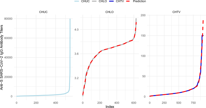
In Fig. 8, we present an example of the application of the aforementioned models, focusing on the specific time point “6 months after vaccination”.

Prediction of anti-SARS-CoV-2 IgG antibody values at the “6 months after vaccination” time point for CHLO and CHTV.
B Data linearization and normalization
A summary of the methods applied for each time point and hospital center is presented in Table 6.
The application of these methods was always followed by mean subtraction and division by the standard deviation.
C Harmonization through quantile interpolation followed by regression for the other time points
C. 1 Post-vaccination
The correlations obtained after linear and cubic interpolation are presented in Table 7.
Cubic interpolation was chosen due to its slightly higher correlation. The result of the cubic interpolation led to the same sample size for both hospital centers. With equal sample sizes in both centers, it was possible to apply Deming regression. The equation obtained for the normalized data is presented in Eq. (15) and graphically illustrated in Fig. 9.
$$\begin{aligned} y = 1.000102 \cdot x + 8.512712 \times 10^{-5} \end{aligned}$$
(15)

Deming regression line for the normalized data between CHUC and CHLO at the “Post-vaccination” time point.
The inverse of the linearization and normalization transformations was applied directly to the fitted equation to recover the original relationship between the data. The normalization values are presented in Table 8.
$$\begin{aligned} & \frac{\sqrt{y’} – a}{b} = 1.000102 \times \frac{(\log _{10}(f – g) – \log _{10}(f – x’)) – d}{e} + 8.512712 \times 10^{-5} \end{aligned}$$
(16)
$$\begin{aligned} & y’ = \left( \left( 1.000102 \times \frac{\left( \log _{10}(f – g) – \log _{10}(f – x’)\right) – d}{e} + 8.512712 \times 10^{-5}\right) b + a\right) ^2 \end{aligned}$$
(17)
C.2 3 months after vaccination
Table 9 presents the results of the interpolation.
Following cubic interpolation, the Deming regression result is shown in Eq. (18) and illustrated graphically in Fig. 10.
$$\begin{aligned} y = 0.9998562856 \cdot x + 3.375096 \times 10^{-9} \end{aligned}$$
(18)

Deming regression line for the normalized data between CHUC and CHLO at the “3 months” time point.
However, as previously mentioned, it is essential to determine the equation to apply it directly to the original data. For this, the normalization values to be applied in the equation are provided in Table 10.
$$\begin{aligned} & \frac{\left( \frac{(y’+1)^{a}-1}{a} \right) -b}{c} = 0.9998562856 \times \frac{\left( \log _{10}(g – h) – \log _{10}(g – x’)\right) – e}{f} – 0.0003375096 \end{aligned}$$
(19)
$$\begin{aligned} & y’ = \left( \left( \left( 0.999\,856\,285\,6 \times \frac{\left( \log _{10}(g – h) – \log _{10}(g – x’)\right) – e}{f} – 0.000\,337\,509\,6\right) c + b \right) a + 1 \right) ^{\frac{1}{a}} – 1 \end{aligned}$$
(20)
12 months – before booster
The correlation results of anti-SARS-CoV-2 IgG antibodies after linear and cubic interpolation are presented in Table 11.
Deming regression was applied to the interpolated data, with the resulting model presented in Eq. (21) and illustrated in Fig. 11.
$$\begin{aligned} y = 0.9989436644 \cdot x – 3.369187 \times 10^{-4} \end{aligned}$$
(21)

Deming regression line on normalized data between CHUC and CHLO at the time point “12 months – Before booster”.
C.4 Post-booster
Calculation of correlations between the hospitals after applying both interpolation methods, with the results shown in Table 12.
Considering the correlation values, cubic interpolation was used for CHUC and linear interpolation for CHTV.
CHLO: For this particular hospital, Eq. (22) was obtained from the application of Deming regression, along with the corresponding Fig. 12.
$$\begin{aligned} y = 0.9991075153 \cdot x + 8.864896 \times 10^{-4} \end{aligned}$$
(22)

Deming regression line between CHUC and CHLO at the “Post-booster” time point.
The conversion of the normalized equation to the corresponding one on the original data scale was then performed. The values required for this conversion are presented in Table 13.
$$\begin{aligned} & \frac{\operatorname {asinh}(y’) – a}{b} = 0.999\,107\,515\,3 \times \frac{\left( \log _{10}(f – g) – \log _{10}(f – x’)\right) – d}{e} + 0.000\,886\,489\,6 \end{aligned}$$
(23)
$$\begin{aligned} & y’ = \sinh \left( \left( 0.999\,107\,515\,3 \times \frac{\left( \log _{10}(f – g) – \log _{10}(f – x’)\right) – d}{e} + 0.000\,886\,489\,6 \right) b + a \right) \end{aligned}$$
(24)
CHTV: For the CHTV hospital, Eq. (25) was obtained based on the normalized data, with the graphical representation shown in Fig. 13.
$$\begin{aligned} y = 0.9985563 \cdot x – 8.868104 \times 10^{-5} \end{aligned}$$
(25)

Deming regression line on normalized data between CHUC and CHTV at the “Post-booster” time point.
Once the equation with normalized data has been determined, it becomes necessary to convert it so that it can be applied to the original data. The normalization values are summarized in Table 14.
$$\begin{aligned} & \frac{\operatorname {asinh}(y’) – a}{b} = 0.9985563 \times \frac{\left( \log _{10}(f – g) – \log _{10}(f – x’)\right) – d}{e} – 8.868104 \times 10^{-5} \end{aligned}$$
(26)
$$\begin{aligned} & y’ = \sinh \left( \left( 0.9985563 \times \frac{\left( \log _{10}(f – g) – \log _{10}(f – x’)\right) – d}{e} – 8.868104 \times 10^{-5} \right) b + a \right) \end{aligned}$$
(27)