Genetics and environment distinctively shape the human immune cell epigenome

Data generation

FACS of immune cell types

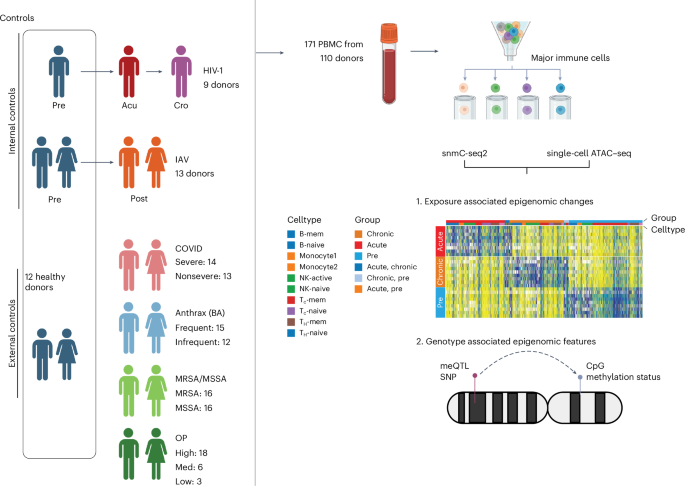
Cells were sorted into 384-well plates using FACS based on their specific antibody labeling. The FACS antibody cocktail allowed for the identification of seven different immune cell types in blood (Extended Data Fig. 1). The sorted cell types included naive helper T cells (CD3⁺, CD4⁺, CCR7⁺, CD45RA⁺), memory helper T cells (CD3⁺, CD4⁺, CD45RA⁻), naive cytotoxic T cells (CD3⁺, CD8⁺, CCR7⁺, CD45RA⁺), memory cytotoxic T cells (CD3⁺, CD8⁺, CD45RA⁻), B cells (CD3⁻, CD19⁺), monocytes (CD3⁻, CD19⁻, CD14⁺), NK cells (CD3⁻, CD19⁻, CD14⁻, CD16⁺, CD56⁺) and other cells (CD3⁻, CD19⁻, CD14⁻, CD16⁻, CD56⁻). The SONY Multi-Application Cell Sorter LE-MA900 Series was used to isolate single cells in 384-well PCR plates containing protein kinase. After cell sorting, the plates were centrifuged to collect the cells at the bottom of the wells, and the wells were then subjected to thermocycling at 50 °C for 20 min. The plates containing the DNA from the cells were subsequently stored at −20 °C or moved directly to library preparation.

snmC-seq2 library preparation and Illumina sequencing

For library preparation, we followed the previously described methods for bisulfite conversion and library preparation in snmC-seq2 (refs. ^14,37). The snmC-seq2 libraries generated from isolated immune cells were sequenced on an Illumina Novaseq 6000 using S4 flow cells in 150-bp paired-end mode. Freedom EVOware (v2.7) was used for library preparation, while Illumina MiSeq control software (v3.1.0.13) and NovaSeq 6000 control software (v1.6.0) and Real-Time Analysis (RTA; v3.4.4) were used for sequencing.

snATAC–seq

snATAC–seq was performed as previously described³⁸, using either the Chromium Next GEM Single Cell ATAC Library & Gel Bead Kit v1.1 (10x Genomics, 1000175) with the Chromium Next GEM Chip H (10x Genomics, 1000161) or the Chromium Single Cell ATAC Library & Gel Bead Kit (10x Genomics, 1000110). Libraries were sequenced on an Illumina NovaSeq 6000 system (1.4 pM loading concentration) using a 50 × 8 × 16 × 49 bp read configuration, targeting an average of 25,000 reads per nucleus.

Quantification and statistical analysis

Single-cell methylation data processing (alignment, quality control (QC))

For alignment and QC of the single-cell methylation data, we used the same mapping strategy used in our previous single-cell methylation projects in our lab³⁹. Specifically, we used our in-house mapping pipeline, YAP (https://hq-1.gitbook.io/mc/), for all the mapping-related analysis. The pipeline includes the following main steps: (1) demultiplexing FASTQ files into single cells with Trim Galore (v4.4), (2) reads-level QC, (3) mapping with bismark (v0.20.0), (4) BAM file processing and QC with samtools (1.17) and Picard MarkDuplicates (v3.0.0), and (5) generation of the final molecular profile. Detailed descriptions of these steps for snmC-seq2 can be found in ref. ¹⁴. All the reads were mapped to the human hg38 genome, and we calculated the methylcytosine counts and total cytosine counts for two sets of genomic regions in each cell after mapping.

We filtered out low-quality cells based on three metrics generated during mapping—mapping rate >50%, final mC reads >500,000 and global mCG >0.5. Chromosomes X, Y and M were excluded from the analysis and the remaining genome was divided into 5-kb bins to create a cell-by-bin matrix. In this matrix, each bin was assigned a hypomethylation score (hyposcore) calculated from the P values of a binomial test, which indicates the probability of hypomethylation of that bin. The matrix was further binarized for downstream analysis using a hyposcore cutoff ≥0.95.

Hyposcore measures the likelihood of observing greater than m methylated reads under the assumption that methylation follows the binomial distribution with parameters c and p.

where m is the observed number of methylated count for region i, c is the coverage (total count) covering region i, n is the total number of 5-kb bin regions and p is the expected probability of methylation for this cell.

Let’s assume

then for each 5-kb bin,

The calculation of hyposcore was implemented in ALLCools (v1.1.1, https://lhqing.github.io/ALLCools/intro.html) using SciPy⁴⁰_.

Bins covered by fewer than five cells and those with any absolute z score (the number of cells with nonzero values) >2 were filtered out. Additionally, we excluded bins that overlapped with the ENCODE blacklist using ‘bedtools intersect’ (Dale, Pedersen and Quinlan 2011; Quinlan and Hall 2010).

Unsupervised clustering

To perform unsupervised clustering, we used ALLCools³⁹, which first conducted PCA on the 5-kb bin matrix. For each exposure, we selected the top 32 principal components (PCs) for clustering using the modules in scanpy. In the HIV-1 and influenza cohorts, we observed a donor effect in the clustering results with these PCs. Therefore, we applied harmony⁴¹ to correct the donor effect on these PCs. We performed clustering separately for control samples (‘HIV_pre’, ‘Flu_pre’ and ‘Ctrl’) and samples from the ‘MRSA/MSSA’, ‘BA’, ‘COVID-19’ and ‘OP’ groups, allowing for better comparison between the exposures and control samples.

To annotate the cells, we used both the single-cell methylation clustering results and cell-surface markers. In almost every cohort, we observed two clusters of B cells and NK cells, which were distinguished by their global mCG levels. Therefore, we assigned these clusters as naive and memory B cells, naive and active NK cells. We also merged clusters with cell-surface markers indicating memory CD4 and CD8 T cells, even if they exhibited multiple clusters in the t-SNE embedding.

eDMRs identification

To identify DMRs associated with each immune cell type, we analyzed PBMCs from healthy donors. Based on single-cell methylation and FACS, we identified nine cell types through clustering. These cell types were grouped based on their global mCG levels, and DMRs were called separately within high-mCG and low-mCG cell types. We used methylpy (v1.4.6, https://github.com/yupenghe/methylpy) for DMR calling and the resulting DMRs were further annotated with genes and promoters.

To identify DMRs associated with each exposure, we merged the control samples and samples from each exposure group. We used methylpy (https://github.com/yupenghe/methylpy) to identify DMRs between the control and exposure groups and between different exposure groups. Once we obtained the primary set of DMRs, we calculated the methylation levels of all samples at these DMRs using ‘methylpy add-methylation-level’.

Additional filtering of the DMRs was performed by comparing methylation levels across sample groups using Student’s t test. Only DMRs with a minimum P value <0.05 between any two groups were retained. For DMRs associated with MRSA/MSSA, BA, OP and SARS-CoV-2, where external controls were used for DMR calling, we compared the methylation levels of exposure samples and control samples, as well as different cohorts of controls (HIV, Flu and commercial controls). DMRs that showed significant differences (P < 0.05) between the exposure group and all three control cohorts, but no significant differences (P > 0.05) between any two control cohorts, were retained.

To visualize complex heatmaps, we used PyComplexHeatmap (https://github.com/DingWB/PyComplexHeatmap)^38,42. Hypomethylated DMRs in the corresponding sample groups and cell types were labeled for better visualization. The heatmap rows were split according to sample groups and the columns were split based on DMR groups and cell types. Within each subgroup, rows and columns were clustered using Ward linkage and the Jaccard metric.

Validation of DMRs by shuffling the samples

To validate that the identified DMRs for each exposure were not confounded by batch effects or other factors, we shuffled the group labels of the samples within each exposure and identified DMRs among the randomly assigned groups. We quantified the methylation levels of all samples at the DMRs from the random groups and performed t tests on the methylation levels between each pair of groups.

Effect-size calculation

To quantify the magnitude of methylation differences across exposure groups, we calculated Cohen’s d effect sizes for each DMR using pairwise comparisons. For each DMR, methylation values were extracted across the three defined groups. Cohen’s d was computed using the pooled standard deviation formula:

where mean₁ and mean₂ are the group means and s_pooled is the square root of the weighted average of group variances. The pooled variance was calculated with Bessel’s correction to account for sample size differences. For each DMR, three pairwise d values were computed—Group1 versus Group2, Group1 versus Group3 and Group2 versus Group3. These effect sizes provide an interpretable measure of methylation divergence independent of sample size or statistical significance.

SNP calling

We merged the BAM files from the same donors and SNP calling was performed using Biscuit’s³² variant calling function. This process identifies SNPs in both CpG and nonCpG contexts by analyzing the bisulfite-treated reads. Biscuit distinguishes between methylated cytosines and actual C/T polymorphisms, reducing the risk of false positives. To increase variant density and coverage, we imputed SNPs using Minimac4, referencing the 1,000 Genomes Phase 3 panel. Postimputation, only high-confidence SNPs present in dbSNP were retained to ensure reliability and compatibility with downstream analyses.

Standard variant filtering was applied to remove low-confidence SNPs. We excluded SNPs with a minor allele frequency (MAF) below 0.05. Additionally, SNPs overlapping with regions in the blacklist were filtered out.

Genetic PCA analysis

We performed PCA of genotypes following standard best practices to control for population structure as follows:

1. 1.

   Linkage disequilibrium (LD) pruning—we used PLINK 2 to filter variants to high-quality, common biallelic SNPs (–snps–only just-a–t, –max-alleles 2, –geno 0.02 and –maf 0.05) and excluded regions of extended LD (high-LD-regions-hg38.bed). We then applied LD pruning with a 200-SNP window, step size of 50 SNPs and an r² threshold of 0.1 (–indep-pairwise 200 50 0.1).

2. 2.

   Preparation of input genotypes—the pruned SNP set was extracted to generate a reduced variant call format (VCF) for PCA, ensuring that only informative and independent variants were retained.

3. 3.

   PCA computation:

   1. (a)

      The primary analysis was conducted using QTLtool with the options –center, –scale, –maf 0.05 and –distance 0, which ensures mean centering, scaling and consistent handling of pruned SNPs.

   2. (b)

      For cross-validation, we also performed PCA with PLINK 2 (–pca 20 approx var-wts), which produced highly concordant results.

This approach ensured robust inference of genetic PCs, minimizing the impact of LD and technical artifacts and provided reliable covariates for downstream QTL and association analyses.

Identification of gDMR–meQTL pairs

To identify meQTLs associated with DMRs, we used QTLtools (v2.0-7-g61a04d2c5e)⁴³. The analysis was conducted using two approaches—nominal and permutation-based methods—both designed to account for the statistical significance of the association between SNPs and methylation levels. DMRs for each cell type were identified across the 110 donors using methylpy.

meQTL mapping

Nominal analysis

We used QTLtools in nominal mode to calculate the association between genotype (SNP) and methylation levels within DMRs. This method tests all SNP–DMR pairs within a specified genomic window (1 Mb) around the DMRs, reporting nominal P values for each pair. Associations were considered significant at an FDR threshold <0.01.

Permutation-based analysis

To assess the bias in the proportion of COVID-19 samples across different monocyte clusters, a chi-square test was applied. This test helped determine whether the distribution of samples from severe and nonsevere COVID-19 patients differed significantly from that of control samples, with results indicating a strong statistical difference (P = 2.05 × 10⁻²³⁷, Fisher’s exact test).

Trans-meQTL mapping

We used TensorQTL in trans mode to efficiently test large-scale genotype–methylation associations. By default, TensorQTL computes parametric P values using linear regression and applies Benjamini–Hochberg FDR correction.

Covariates and adjustment

In both analyses, we included covariates such as age, sex, the first five PCs of genotypes and exposures. Covariate adjustment was performed using the QTLtools built-in method for linear model regression.

Motif enrichment

We obtained the hypo- and hyper-DMRs reported by methylpy from the columns ‘hypermethylated_samples’ and ‘hypomethylated_samples’. HOMER (v5.1) was used to identify enriched motifs within these different sets of DMRs for each exposure. The results from HOMER’s ‘knownResults.txt’ output files were used for downstream analysis. Only motif enrichments with a P value <0.01 were retained. Motif enrichment results were visualized using scatter plots generated with Seaborn.

DMG identification

Pairwise DMG analysis for each exposure was performed using ALLCools, following the tutorial (https://lhqing.github.io/ALLCools/cell_level/dmg/04-PairwiseDMG.html). Significantly DMGs were selected based on an FDR < 0.01 and a delta mCG > 0.05. The functional enrichment analysis of the DMGs was conducted using Metascape⁴⁴ (v3.5, https://metascape.org/). We also used linear regression (mCG ~ annotation + age + sex + ethnicity) to identify the genes associated with the two clusters of monocytes, regressing out age, sex and ethnicity of the donors.

Integration with single-cell ATAC

We integrated our single-cell methylation data with single-cell ATAC–seq data from HIV-1. This integration was performed using canonical correlation analysis based on 5-kb bins, where we transferred our methylation cell annotations to the cells from the other modality. To generate the peaks and BigWig files for each cell type, we used SnapATAC2 (refs. ^45,46).

Correlation of single-cell methylation and single-cell ATAC

To assess the correlation between single-cell methylation and single-cell ATAC, we calculated the correlation between the hyposcore of each 5-kb bin and Tn5 insertions in each bin. This correlation was performed both across different cell types and within matched cell types.

Colocalization of meQTL with GWAS traits

Summary statistics of GWAS were downloaded from the NHGRI-EBI GWAS Catalog (https://www.ebi.ac.uk/gwas/)⁴⁷, including 29,401 studies and 25,111 traits. We performed colocalization analysis with coloc⁴⁸ (v5.2.3) using default priors to calculate the probability that both the meQTL and GWAS traits share a common causal variant. The posterior probability (PP4) of a single causal variant associated with both DMR and GWAS traits was used to identify significant colocalizations (PP4 > 0.50). A high PP4 value indicates strong evidence for shared causality. R packages locuscomparer (v1.0.0)⁴⁹ and locuszoomr (v0.3.1)⁵⁰ were used to visualize the colocalization results. To assess whether meQTL and GWAS SNPs were significantly overlapping for each DMR–trait pair, we performed chi-squared tests using the ‘stats.chi2_contingency’ function from the Python package SciPy⁴⁰. Resulting P values were adjusted for multiple testing using the Benjamini–Hochberg method.

SMR analysis

To investigate the relationship of eDMRs and gDMRs on gene expression, we performed SMR (v1.0) analysis³⁴ by integrating our unfiltered meQTLs with the eQTLs derived from whole-blood gene-expression levels generated from the eQTLGen consortium^34,51.

By setting the exposure as DMR and outcome as gene expression in the SMR analysis, we tested whether genetic variants associated with DMRs are also associated with expression levels of nearby genes, providing evidence for associations between the two. We did not conduct HEIDI analysis due to the differences between the two sample populations. This does not rule out the possibility that some of the DMR–gene associations identified in our SMR analysis are due to linkage rather than pleiotropy or causality. SMR associations with a P value below the Bonferroni-adjusted alpha level (α = 0.05/n) were considered significant. Default parameters were used to run SMR. We further filtered out associations in the HLA region (chr6: 28,477,797–33,448,354).

Statistics

Enrichment tests

Enrichment tests were conducted using Fisher’s exact test to evaluate the distribution of DMRs across exposures and cell types. This statistical approach was selected due to the small sample sizes in some groups and the need for exact calculations without relying on large-sample approximations.

Bias analysis of COVID samples in monocyte clusters

To assess the bias in the proportion of COVID-19 samples across different monocyte clusters, a chi-square test was applied. This test helped determine whether the distribution of samples from severe and nonsevere COVID-19 patients differed significantly from that of control samples, with results indicating a strong statistical difference (P = 2.05 × 10⁻²³⁷, Fisher’s exact test).

Effect-size calculation

For each DMR, effect sizes were calculated using Cohen’s d to quantify the magnitude of methylation differences among exposure groups. This measure allows for an understanding of the biological relevance of the observed methylation changes, independent of sample size. Cohen’s d was computed for pairwise comparisons across groups (for example, exposure versus control), using the pooled standard deviation formula.

Differential methylation analysis

We performed pairwise differential methylation analysis between exposure groups using the methylpy package. Statistical significance was determined by calculating P values for each comparison, with a threshold of 0.05. Further, we applied FDR correction to adjust for multiple comparisons.

Ethics

The study was conducted with approval from the Salk Institutional Review Board (IRB) under protocol 18-0015 titled ’Single Cell Analysis for Forensic Epigenetics (SAFE)’. Research activities were covered under Salk’s Federalwide Assurance (FWA) for the Protection of Human Subjects (FWA00005316).

Reporting summary

Further information on research design is available in the Nature Portfolio Reporting Summary linked to this article.