Laser interstitial thermal therapy and adjuvant pembrolizumab in recurrent high-grade astrocytoma: a Phase 1/randomized Phase 2b trial

Study design and treatments

Approval

Human subject work was performed in accordance with an approved protocol by the respective internal review boards at the Washington University in St. Louis School of Medicine, the University of Florida College of Medicine, and the University of Southern California Keck School of Medicine, in accordance with the Declaration of Helsinki. A written informed consent was obtained from each human participant before study procedures and analysis were performed. All enrollments were completed at Washington University and the University of Florida. The correlative analysis was performed at the University of Southern California. The study’s ClinicalTrials.gov identifier number is NCT02311582.

Study design

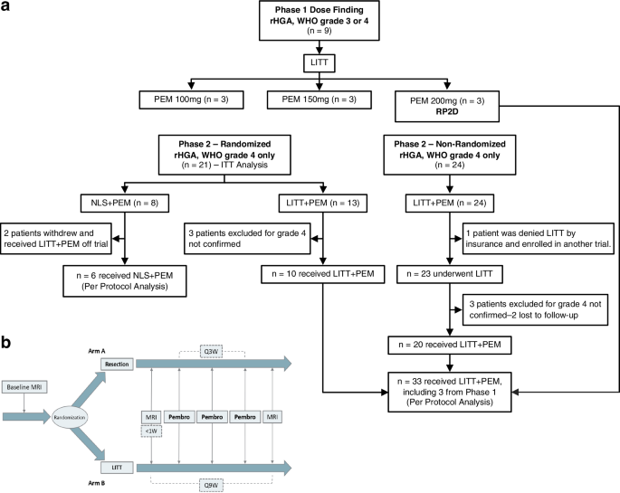
The study began with a Phase 1 lead-in to assess pembrolizumab safety in rHGA, followed by a randomized Phase 2 at a ratio 1:1 comparing NLS + PEM to LITT + PEM in rHGA. Randomization was computer-generated using a blocked scheme generated in SAS (v9.3+) and conducted centrally via the electronic data capture system REDCap. After emerging data demonstrated the limited benefit of ICI monotherapy in recurrent GBM (ClinicalTrials.gov, NCT02337491)⁵, the independent Data and Safety Monitoring Committee (DSMC) requested an unscheduled interim review of accumulating efficacy data. On the basis of this review, the DSMC recommended closing the NLS + PEM arm and redirecting all subsequent enrollment to LITT + PEM (Protocol Amendment 12). Patients assigned to LITT + PEM could undergo optional surgical debulking prior to LITT; if resection was performed, the laser ablation then targeted only the residual tumor. To bolster our control framework and isolate LITT’s effects without ICI, we then introduced a contemporaneous historical control (CHC) cohort treated with LITT plus non-ICI therapies (LITT+Non-ICI; Table 1). The primary interventions were LITT or NLS followed by adjuvant pembrolizumab, initiated within 1-week post-procedure (Fig. 1b). Patients receiving at least one dose of pembrolizumab were evaluable for survival and response analyses.

Patient population

Between May 2016 and May 2017, nine patients with radiographically recurrent WHO grade 3 or 4 astrocytoma were enrolled in the Phase 1 dose-escalation (3 × 3) cohort, receiving pembrolizumab at 100 mg, 150 mg, or 200 mg IV every 3 weeks following LITT (three patients per dose level). In Phase 2, from January 2017 to December 2022, 45 patients with histologically confirmed recurrent WHO grade 4 astrocytoma enrolled: 21 in the randomized cohort and 24 assigned to LITT + PEM after Amendment 12 (Fig. 1a). Key inclusion criteria were unequivocal tumor progression by RANO, a minimum of 12 weeks from frontline chemoradiation, a candidate for LITT or surgical resection, and Karnofsky performance status (KPS) ≥ 60%. Patients with suspected secondary WHO grade 4 astrocytoma—those with prior grade 2 or 3 tumors treated with chemoradiation, now with radiographic changes suggestive of transformation to grade 4—were conditionally enrolled and received pembrolizumab only after histopathological confirmation of grade 4 post-LITT or post-NLS. Key exclusion criteria included dexamethasone >4 mg/day at registration, prior immunotherapy (anti–PD-1/PD-L1 or anti-CD137), and bilateral multifocal or leptomeningeal disease. IDH mutation and multiple prior recurrences were permitted in both phases (Table 1).

Contemporaneous historical controls

We identified contemporaneous control patients treated at Washington University School of Medicine between 2016 and 2022 for histologically confirmed rHGA via retrospective chart review (see Supplementary Fig. S1a for the schema and criteria). Inclusion criteria mirrored those of the prospective study and required biopsy-confirmed recurrence. We excluded patients with newly diagnosed grade 4 astrocytoma, those enrolled in other LITT trials, and individuals receiving immunotherapy. Of 122 rHGA patients treated with LITT during this period, 13 met all eligibility criteria.

Laser interstitial thermal therapy

LITT is an FDA-cleared, minimally invasive technique for thermal ablation of brain lesions. In our study, we employed the Monteris NeuroBlate Laser Ablation System (Minnetonka, MN) under MRI guidance. Following a small scalp incision and cranial burr hole, an MRI-compatible laser probe is advanced into the tumor. The system then delivers thermal energy, raising the lesion core temperature to ≈70 °C to induce coagulative necrosis, while peritumoral temperatures gradually climb to a peak of 40–45 °C, thereby limiting collateral injury^18,19,20,21.

Statistical analysis plan for clinical and survival comparisons

Phase I: A traditional 3 + 3 design was used to determine the recommended Phase 2 dose of pembrolizumab when combined with LITT for the treatment of rHGA.

Phase 2: The primary endpoint was progression-free survival (PFS); secondary endpoints were overall survival (OS), safety, objective response rate, and immune-response signatures. In both the randomized intent-to-treat and per-protocol cohorts, PFS and OS were measured from first pembrolizumab dose to radiographic progression (per RANO) or death. For the contemporaneous historical control (LITT+non-ICI), both endpoints were calculated from the date of LITT. Patients lost to follow-up or alive at data cutoff were censored at their last known alive date or at cutoff, whichever came first.

Initial Phase 2b calculations (one-sided α = 0.15) assumed six-month PFS of 40% in the NLS + PEM arm—based on published rates (<10–30%) for common salvage regimens such as bevacizumab, temozolomide, carboplatin, carmustine, lomustine, etoposide, irinotecan^{50,51,52,53,54}—and 65% in LITT + PEM, requiring 17 patients per arm for 80% power; we thus targeted 20 per arm. Randomization was not stratified by IDH mutation, MGMT promoter methylation, or other baseline factors because this planned small sample size did not permit reliable balance across multiple strata. After 21 randomized patients, emerging data showing limited ICI monotherapy benefit prompted the independent DSMC to request an unscheduled interim review of the accumulating trial data. This interim analysis was not prespecified in the original protocol and did not use a formal alpha-spending or stopping boundary. Descriptive comparisons at that time indicated longer PFS and OS in the LITT + PEM arm, and, together with the external evidence, led the DSMC to recommend closing the NLS + PEM arm and continuing the trial as a single-arm LITT + PEM extension in the spirit of minimizing harm, potential or perceived, to subjects and to complete the study in a timely manner. Under Amendment 12, the control arm closed, and the trial continued as a single LITT + PEM cohort. For this extension, we conservatively used a 2.9-month median PFS for the NLS + PEM arm (the upper 95% confidence bound rather than the 2.4-month median reported)¹¹. Under that assumption, enrolling 27 additional patients (to achieve 20 evaluable GBM cases) provided 80.9% power (two-sided α = 0.05, one-sample log-rank) to detect an increase in median PFS to 5.1 months versus the 2.9-month benchmark.

In the final analysis, we descriptively compared the PFS distribution of the per-protocol LITT + PEM group, estimated by Kaplan–Meier with its 95% confidence interval, to this 2.9-month benchmark. Two-sample log-rank tests comparing LITT + PEM with NLS + PEM in the randomized ITT and per-protocol populations, and with the contemporaneous LITT+non-ICI cohort, were performed as exploratory analyses to contextualize the magnitude of effect and do not preserve the nominal type I error. Kaplan–Meier curves for OS and PFS were generated with log-rank tests for these unadjusted comparisons. Univariate and multivariable Cox proportional-hazards models adjusted for age, sex, IDH mutation, MGMT methylation, enrolling center, baseline KPS, and number of prior recurrences provided hazard ratios (HR) with 95% confidence intervals and p-values. All tests were two-sided at α = 0.05. Analyses were performed in SAS v9.4 (Cary, NC).

Tumor tissue processing and analysis

All available tumor samples from the study participants that remained after clinical diagnostics were prioritized for whole-exome sequencing and, when sufficient material was left, bulk RNA-seq. Exploratory analyses of intratumoral PD-L1 expression by immunohistochemistry were prespecified but could not be completed in a sufficient number of cases because most biopsies were very small and were exhausted by diagnostic testing and other genomic assays. Only five tumors (three NLS + PEM and two LITT + PEM) had adequate material for bulk RNA-seq–based estimation of PD-L1 expression.

Single cell RNA-seq (scRNA-seq) analysis of PBMCs

Portions of the following scRNA-seq methods are adapted from our prior work³⁰, published under a Creative Commons license, CC BY 4.0, and are included here in full for completeness:

Sample processing

Cryopreserved PBMCs obtained from the study participants were rinsed in PBS, and cell viability was assessed using Trypan Blue staining. Single-cell suspensions were then prepared and applied to the Chromium Single Cell Chip (10x Genomics) as per the instructions provided by the manufacturer. Subsequently, single-cell RNA-seq libraries were generated using the Chromium Next GEM Single Cell 5′ v2 (Dual Index). To ensure consistency, all patient samples and the corresponding libraries were processed simultaneously in a single batch. Sequencing of the single-cell libraries was performed on an Illumina NovaSeq system, utilizing an 8-base i7 sample index read, a 28-base read 1 for capturing cell barcodes and unique molecular identifiers (UMIs), and a 150-base read 2 for the mRNA insert.

Data processing

The main operations were performed using the Seurat R package (3.2.2)^33,34, unless otherwise stated. When option parameters for the function deviated from the default values, we provided details of the changes accordingly. Most of the changes to the default options were made to accommodate and leverage the large size of the dataset. Cell Ranger Aggregation: The raw sequencing data were processed using cellranger mkfastq and cellranger multi commands of the Cell Ranger package as described in the TCR clonotyping section. Results from all libraries and batches were pooled together using the command cellranger aggr without normalization for dead cells, as it will be handled downstream. The filtered background feature barcode matrix obtained from this step was used as input for sequential analysis. Normalization of UMI: Using the global scaling normalization method, the feature expression for each cell was divided by the total expression, multiplied by the scale factor (10,000), and log transformed using the Seurat R function NormalizeData with method “Log Normalize”. Seurat aggregation and correction for batch effect: As the counts were from two different batches, to align cells and eliminate batch effects for dimension reduction and clustering, we adopted the multi-dataset integration strategy as previously described³⁴. Briefly, “anchors cells” were identified between pairs of datasets and used to normalize multiple datasets from different batches. We chose a reference-based, reciprocal PCA variant of the method detailed in the Seurat R package^33,34. First, the previously integrated dataset was split by batches using the Seurat function SplitObject. Next, for each split object, variable features were selected using the function FindVariableFeatures. Features for integration were selected using the function SelectIntegrationFeatures, and PCA performed for each split object on the selected features. The anchor cells were identified by using the function FindIntegrationAnchors with the reference chosen as the largest among two batches and the reduction option set to “rpca”. Finally, the whole datasets from the two batches were reintegrated using the function IntegrateData with the identified anchor cells.

Uniform manifold approximation and projection (UMAP) dimension reduction

The integrated multiple batch dataset was used as input for UMAP dimension reduction³⁵. The feature expression was scaled using the Seurat function ScaleData, followed by a PCA run using the function RunPCA (Seurat) with the total number of principal components (PC) to compute and store option of 100. The UMAP coordinates for single cells were obtained using the RunUMAP function (Seurat) with the top 75 PCs as input features (dims = 1:75) with min.dist = 0.75 and the number of training epochs n.epochs = 2000. Clustering of cells: We relied on a graph-based clustering approach implemented in the Seurat package, which embeds cells in a K-nearest neighbor graph with edges drawn between similar cells and partitions nodes in the network into communities. Briefly, a Shared Nearest Neighbor graph was constructed using the FindNeigbhors function with an option dimension of reduction input dims = 1:75, error bound nn.eps = 0.5. This function calculates the neighborhood overlap (Jaccard index) between every cell and its k.param nearest neighbors⁵⁵. The graph was partitioned into clusters using the FindClusters function with different values for the resolution parameter. The differential expressed gene markers for each cluster were found using the FindAllMarkers function with the option of only returning positive markers and a minimal fraction of cells with the marker of 0.25. The default Wilcoxon Rank Sum test was used to calculate statistical differences in each cell cluster. Alternative 2D embeddings, including t-SNE, were evaluated using quantitative metrics of within-cluster compactness, between-cluster separation, k-nearest-neighbor purity, silhouette width, and kNN-graph modularity, and UMAP most faithfully preserved the predefined clusters and trajectories; UMAP embeddings were therefore used for visualization and as the feature space for downstream distance-based analyses.

Cell type annotation

To delineate specific cell types within the data, cell type labels were assigned manually to clusters emerging from UMAP analysis. This annotation process was guided by the expression profiles of a set of marker genes, which are characteristic of various cell types including T cells, B cells, natural killer (NK) cells, monocytes, dendritic cells (DCs), myeloid-derived suppressor cells (MDSCs), megakaryocytes, red blood cells (RBCs), CD34⁺ stem cells, granulocytes, lymphocytes, macrophages, basophils, eosinophils, and neutrophils. The marker genes utilized for this purpose encompassed a wide range of immune response and cell differentiation indicators such as CD3D, CD3E, ID3, IL7R, CCR7, ITGB1, CD95, TCF7, CD3D, CD3E, CD4, S100A4, CCR10, FOXP3, IL2RA, TNFRSF18, IKZF2, CTLA4, IL2, IL4, IL13, IL17A, CD3D, CD3E, CD8A, CD8B, CCL4, GZMA, GZMB, GZMH, GZMM, GZMK, IFNG, GNLY, TNF, PDCD1, LAG3, CD79A, CD79B, CD19, JCHAIN, GNLY, NKG7, CD16, NCAM1, KIR2DL4, SIGLEC7, CD14, LYZ, S100A8, S100A9, LGALS3, FCN1, FCGR3A, MS4A7, FCER1A, CST3, ITGAM, ITGAX, CLEC10A, CLEC9A, THBD, CD1C, LILRA4, CLEC4C, TLR7, TLR9, ITGAM, CD33, CD3D, CD3E, CD14, CD19, FUT4, CEACAM1, HLA-DRA, HLA-DRB1, HLA-DRB5, PPBP, PF4, ITGA2B, ITGB3, PEAR1, CD42D, CD59, HBG1, HBG2, HBB, CD34, CCR3, CD11b, CD13, CD18, CD229, CRACC, CD14, CD68, CD36, CD164, LAMP1, CD44, CD69, EMR1, MPO, CD62L, CD3D, CD3E, CD4, CD8A, CD8B, NKG7, GNLY, CD14, LYZ, FCER1A, CLEC10A, LILRA4, CLEC4C, CD79A, CD79B, HBB, PPBP, and PF4. T cells were further divided into clusters to annotate subpopulations: naive CD4, central memory CD4, central memory CD8, anergic CD4, activated CD4, Treg, exhausted CD4, stem-like CD8, NKT, exhausted CD8, effector CD8, naive CD8, cytotoxic CD4, and effector memory CD8 using the following marker genes: CD3D, CD4, CD8A, CTLA4, PDCD1, TIGIT, FOXP3, CCR7, GZMK, GZMB, GZMH, IL7R, CCL5, KLRB1, TRAV16, TRAV17, CX3CR1, CCL4, TRDC, CD69, FOS, BATF, IL2RB, TBX21, EOMES, PRDM1, and ICOS. Monocyte cells were further divided into classical and non-classical monocytes using the following marker genes: CD14, IRF8, CCR2, CX3CR1, and FCGR3A.

Differential expression analysis

To evaluate transcriptomic changes in non-classical monocytes between the Pre-LITT and C1 timepoints from the LITT + PEM cohort, a differential expression (DE) analysis was performed using an aggregated “pseudo-bulk” RNA-seq approach, followed by heatmap visualization of the top differentially expressed genes:

• Pseudo-bulk aggregation: the Seurat object was subset to retain non-classical monocyte cells at the Pre-LITT and C1 timepoints. For each patient and timepoint, the raw count data were summed across all cells in that group, yielding a pseudo-bulk expression profile (\({genes}\times {samples}\)). By using this aggregation strategy, cell-level biases are circumvented, and an approximation of bulk RNA-seq at the patient–timepoint level is achieved.

• Differential expression with edgeR:

1. a.

   A DGEList object was created from the aggregated counts.

2. b.

   Normalization factors were computed via calcNormFactors.

3. c.

   A design matrix was constructed (\(\sim {Patient}+{TimePoint}\)) to compare Pre-LITT vs. C1.

4. d.

   After dispersion was estimated, a negative binomial model was fit, and likelihood ratio tests (glmLRT) were performed.

5. e.

   The resulting DE table was filtered for significance, capturing log₂ fold change (log₂FC) and FDR values.

• Top-gene selection and visualization: The top 500 differentially expressed genes by FDR were selected for further inspection. To highlight variation among patients, the log₂FC (Pre-LITT vs. C1) were transformed into z-scores, and these scaled values were visualized in a heatmap. The heatmap columns were ordered according to patient survival times, thus facilitating a direct comparison of expression patterns across different clinical outcomes.

Z-score calculation and GSEA ranking

In the non-classical monocytes of the Experimental group, gene expression differences between time point Pre-LITT and time point C1 were assessed using log₂FC values. For each gene, the mean log₂FC was calculated separately for the short-term group (\({\overline{x}}_{S}\))—LITT + PEM (\({\overline{x}}_{L}\))—LITT + PEM (>mOS). The sample standard deviations (SD) were estimated for each group, and the number of patients in each group was denoted as \({n}_{S}\) (short-term or \({n}_{L}\) (long-term or > mOS).

A z-score was then computed to represent the difference between the two groups using the following equation:

where \({{x}_{\_}}_{L}-{{x}_{\_}}_{S}\) indicates the difference in mean log₂FC [(>mOS) minus (mOS) survivors, whereas negative z-scores are indicative of higher expression in LITT + PEM (

GSEA for pathway identification and confirmation

Based on the z-scores computed as described above, a set of the top 500 differentially expressed genes by the lowest FDR was identified. This subset of genes, showing the most statistically significant differences between the Pre-LITT and C1 timepoints in non-classical monocytes in the LITT + PEM cohort, was treated as a custom gene set of interest. To further elucidate the biological pathways that may be driving survival differences, GSEA was performed using two inputs: (i) the ranked list of all genes (ordered by descending z-score), and (ii) the newly defined custom gene set of 500 genes. Following the standard procedure, GSEA was carried out by using the ranked list to calculate an enrichment score (ES), which reflects the degree to which the custom gene set is overrepresented at either the top (positive z-scores) or the bottom (negative z-scores) of the ranked list. Statistical significance was assessed by permuting the gene labels and recalculating the ES to generate a null distribution. This permitted estimation of the nominal P-value and the FDR q-value for enrichment.

Cox proportional hazard model for survival prediction using the identified GSEA gene set

The scaled and normalized log₂FC of the top 500 genes by FDR was tested as a predictor of overall survival, beyond known clinical factors such as patient age, in a Cox proportional hazards model. First, the scaled and normalized log₂FC of these 500 genes for each patient was summarized by taking the mean across the genes for each individual patient. Then, a binary covariate was created by categorizing patients into “high” or “low” expression groups based on the median of this summarized value for the cohort. This binary pathway-expression variable was combined with age (a continuous variable) as a covariate to determine whether patients with pathway-expression values above the median had a statistically different hazard ratio (i.e., risk of death or relapse) compared with those whose expression was below the median, after adjusting for age. The resulting hazard ratio and its confidence interval provided an estimate of how strongly pathway expression correlates with survival outcomes. The Schoenfeld residuals test⁵⁶ was used to assess the proportional hazards assumption in the Cox regression model, and no covariates demonstrated significant violation, indicating that the assumption held for the model.

Pathway activity signal change comparison

To compare pathway activity changes between NLS + PEM and LITT + PEM arms across consecutive timepoints, T-cell subpopulations were first defined based on clustering annotations derived from the Seurat workflow. For each pathway of interest (specified in a GMT file), the relevant genes were extracted, and the average expression of those genes computed within each patient and time point. Specifically, the following steps were performed:

• Pathway Gene Extraction: A GMT file containing predefined pathways was parsed to identify the set of genes corresponding to each pathway.

• Subset and Normalization: For each T cell subpopulation, a subset of the Seurat object was created. Expression values were normalized using the relative counts (RC) method (normalization.method = “RC” with a scale factor of \({10}^{6}\)).

• Mean Pathway Expression: For each patient and time point, the mean expression of the pathway genes in the corresponding subpopulation was computed.

• Ratio-Based Change Computation: To quantify the relative fold change in pathway activity between two consecutive timepoints (A and B), the ratio of mean pathway expression at timepoint B to the mean pathway expression at timepoint A was used:

• Statistical Assessment: For each comparison, the ratio values for the NLS + PEM and LITT + PEM arms were pooled, and a Wilcoxon rank-sum test was performed to evaluate differences between arms.

All comparisons were repeated across the T cell clusters of interest and for the two pathways, T Cell Activation (GO: 0042110) and Adaptive Immune Response (GO: 0002250), defined in the GMT file. Figures were generated to visualize both the per-patient longitudinal changes (line plots) and the distribution of ratio values by treatment arm (box plots).

TCR clonotyping

Portions of the following TCR clonotyping methods are adapted from our prior work³⁰, published under a Creative Commons license, CC BY 4.0, and are included here in full for completeness:

Sample processing

Single-cell RNA-seq libraries were generated using the Chromium Next GEM Single Cell 5′ v2 (Dual Index) alongside the Human V(D)J Amplification Kit (10x Genomics), following the manufacturer’s protocols. To ensure consistency, all patient samples and the corresponding libraries were processed simultaneously in a single batch. Sequencing of the single-cell libraries was performed on an Illumina NovaSeq system, utilizing an 8-base i7 sample index read, a 28-base read 1 for capturing cell barcodes and unique molecular identifiers (UMIs), and a 150-base read 2 for the mRNA insert.

Data processing

The 5′ single cell TCRα/β V(D)J library data were first processed using the 10x Genomics Cell Ranger package (v.7.0.0, with Java/9.0.1, bcl2fastq/2.20.0.422 dependencies). Command cellranger mkfastq was used to convert the raw sequencing data from the bcl to fastq format, and the cellranger multi command to align to the reference genomes GRCh38 (GENCODE v.24) and single cell clonal identification. Clonal tracking plots were created using the Immunoarch R package v0.9.0 (https://cloud.r-project.org/web/packages/immunarch/index.html) with the function trackClonotypes, option col = ”a.a” to collapse all clones that share the same amino acid sequences.

TCR clonotyping, diversity, and evolution

A clonal tracking grid was established to map the presence and characteristics of TCRβ clones at each patient timepoint, focusing on aspects such as the number of cells, changes in cell type, and pathway activity.

• Clonal Diversity by Simpson Index: All unique TCRβ clones in the CD8 T cell subset were first identified for each patient. The Simpson diversity index, \(D\), was then defined as:

where \({p}_{i}\) is the proportion of cells belonging to clone \(i\), and \(n\) is the total number of unique clones within a patient’s T cell repertoire. Lower values of \(D\) indicate reduced diversity (i.e., fewer clones dominate the repertoire), reflecting a higher degree of clonal expansion. Conversely, higher values of \(D\) signify a more evenly distributed clonal landscape. Thus, this index measures the probability that two randomly selected individuals from the population will be of the same clone, with values ranging from zero (no diversity) to one (maximum diversity). This ratio provides a comparative measure of clonal diversity between two specified timepoints. A ratio greater than one indicates an increase in diversity, suggesting a diversification of the clonal population over time. Conversely, a ratio less than one reflects a decrease in diversity, pointing to a homogenization of the population. This analysis facilitates the understanding of clonal dynamics over the course of the study.

The corresponding \(P\)-values were calculated under the null hypothesis that the mean diversity of the two cohorts does not differ significantly. A low \(P\)-value (\(P < 0.05\)) indicates that one cohort exhibits a statistically different clonal diversity—and thus a different degree of clonal expansion—relative to the other.

Tracking T cells Clones Across Timepoints

An Optimal Transport (OT) algorithm^37,38 was used to trace CD8 T-cell clones between consecutive timepoints across three  cohorts [NLS + PEM, LITT + PEM (mOS)]. The analysis quantified how individual T-cell subpopulations (e.g., effector CD8⁺, exhausted CD8⁺ T cells) transitioned at both single-cell and cluster levels from one timepoint to the next. The steps were as follows:

• Data Preparation and Subset Selection: For each cohort and T cell subpopulation, single-cell expression and UMAP coordinates were collected at each available timepoint (e.g., Pre-Procedure, C1, C2, C4, etc.). Clusters of particular interest (COI) were merged where necessary to reduce sparsity.

• Cost Matrix Construction for OT: For each pair of consecutive timepoints, a cost matrix was computed based on Euclidean distances in principal component (PC) space. Let \({x}_{i}\) and \({y}_{j}\) be the PC embeddings for cell \(i\) in the source timepoint and cell \(j\) in the target timepoint, respectively, with the cost defined as:

Uniform distributions \(a\) and \(b\) were imposed over the source and target cells, respectively, ensuring equal weights for all cells.

• Computing the OT Plan: The OT plan \({\pi }{*}\) was solved via the Earth Mover’s Wasserstein Distance (ot.emd) function:

  $${\min }_{\pi \ge 0}{\sum }_{i,j}{\pi }_{{ij}}{C}_{{ij}}{subject\; to}{\sum }_{j}{\pi }_{{ij}}={a}_{i},{\sum }_{i}{\pi }_{{ij}}={b}_{j}.$$

  (5)

  The resulting \({\pi }{*}\) yields a principled “cell-to-cell matching” under global cost minimization.

• UMAP-based Visualization: Using the final OT plan, each source cell was mapped to a corresponding target cell, and arrows were plotted in UMAP coordinates:

• Single-Cell Arrows: Each source cell had an arrow drawn to its corresponding target cell. Down-sampling was carried out to ensure consistent cell counts for plotting.

• Cluster-Level Arrows: By aggregating source and target coordinates within each cluster, representative arrows were drawn for each cluster of interest.

• Aggregated Arrow: Summed cluster displacements produced a single arrow reflecting the global population shift between two timepoints.

• Stacked-Bar Distributions: For each COI, the fractions of its cells in the source timepoint that mapped to each possible target cluster were computed. These fractions were represented as stacked bar charts, illustrating cluster transition patterns over successive timepoints.

• Cohort Comparisons: This pipeline was repeated for all T cell subpopulations across the three cohorts [NLS + PEM, LITT + PEM (mOS)], enabling direct comparisons of clonal dynamics. Variations in both the directional shifts (arrows) and target cluster memberships (stacked bars) offered insight into how clonal populations evolved under different experimental conditions.

Target distribution of T cell clones across timepoints

Following the determination of how each source T cell mapped to a target cluster, cohort-specific target distributions were compared to assess whether different cohorts yield distinct post-mapping cluster compositions. Specifically, for each cohort (e.g., NLS + PEM vs. LITT + PEM), the frequency with which source T cells, which were drawn from one timepoint and mapped to various clusters at the subsequent timepoint, was counted. These counts were then organized into a contingency table, where rows represented target clusters and columns represented cohorts.

Once the contingency table was constructed, a Chi-square test of independence was performed to determine whether the observed target cluster distributions differed significantly across cohorts. A low \(P\)-value (e.g., \(P < 0.05\)) indicated that the distribution of mapped target clusters was not independent of cohort membership, i.e., there was evidence to suggest that different cohorts lead to different cluster-level outcomes for T cells across timepoints. Conversely, a higher \(P\)-value implied that the observed distribution of target clusters could be attributed to chance alone, indicating no statistically significant difference between cohorts in their target distributions.

Immune checkpoint expression comparison

To visualize immune checkpoint expression at multiple timepoints across three cohorts [NLS + PEM, LITT + PEM (mOS)], a set of genes of interest (e.g., PDCD1, CD274, IDO-1) was defined, and FeaturePlot- and density-based visualizations were then generated as follows:

• Data Preparation and Cohort Assignment: Patients were first classified into three cohorts [NLS + PEM, LITT + PEM (mOS)] based on OS. A Seurat object containing T-cell data was filtered to include only those patients overlapping with the survival dataset. The metadata was updated with a SurvivalGroup label for each cell, enabling straightforward subgroup analyses.

• Timepoint Filtering and Down-sampling: Analyses were restricted to timepoints Pre-Procedure, C1, and C2, discarding cells from other timepoints. To avoid uneven sampling, each cohort was down-sampled at each timepoint to ensure approximately equal cell counts, thereby reducing biases introduced by disproportional representation.

• Split Panel FeaturePlots: For each immune checkpoint gene, FeaturePlot was used to visualize expression on UMAP embeddings. The data were split by both cohort and timepoint (i.e., Group_TimePoint), resulting in subplots such as NLS + PEM_Pre-NLS, NLS + PEM_C1, and so forth. Each subplot included cells for the relevant subgroup and colored them according to the expression level of the target gene.

• 2D Density Plots for High Expressors: In parallel, 2D density plots were generated to highlight cells with high (e.g., top 10% or 50%) expression of each gene. These top-expressing cells were colored by cohort, allowing comparisons of the spatial distribution of strongly expressing cells across cohorts within the UMAP space. Specifically, geom_density_2d was applied in ggplot2, with expression values used as weights, thus reflecting how each subgroup’s high-expressing cells cluster or disperse.

Reporting summary

Further information on research design is available in the Nature Portfolio Reporting Summary linked to this article.