
Sample collection
Respiratory tract tissues (trachea and lung) and intestinal tissues (small and large intestine) from three healthy, 3-year-old, crossbred Holstein-Angus steers were included in this study. Samples were collected from the Iowa State University Meat Laboratory during the routine slaughtering process for meat. Tissues were fixed in 10% neutral buffered neutral formalin and then embedded in paraffin blocks. Sections were sliced at 4 μm thickness, transferred onto glass slides (VWR International, Radnor, PA, USA), and prepared for analysis. Lectin staining was used to demonstrate sialic acids, and an indirect immunofluorescence assay was used to detect coronavirus receptors.
For antigen retrieval, deparaffinized slides were treated with 10 mM sodium citrate buffer (pH 6.0; Millipore-Sigma, Burlington, MA, USA) at 96 °C for 30 min, then washed three times with Tris-buffered saline containing 0.1% Tween 20 (TBST; Millipore-Sigma).
Lectin staining
Plant lectins from Sambucus nigra (SNA), Maackia amurensis (MAL-I and MAL-II) were used to detect α2,6-linked SA, SA α2,3-Gal-β (1–4) GlcNAc and SA α2,3-Gal-β (1–3) GalNAc, respectively. To block non-specific binding, tissue sections were incubated with Carbo-Free™ Blocking Solution (Cat# SP-5040-125, Vector Laboratories, Burlingame, CA, USA) for 30 min at room temperature (21–22 °C). Endogenous biotin, biotin receptors, and streptavidin binding sites in tissues were blocked by incubating with biotin and streptavidin solutions (Cat# SP-2002, Vector Laboratories) for 10 min at room temperature.
The sections were then incubated overnight (16 h) at 4 °C in a humidified chamber with optimized concentrations of 10 µg/ml fluorescein isothiocyanate (FITC) labeled SNA (Cat# FL-1301-2, Vector Laboratories) or 10 µg/ml FITC labeled MAL I (Cat# FL-1311-2, Vector Laboratories), and 5 µg/ml MAL II (Cat# B-1265-1, Vector Laboratories). After three washes with TBST, the sections were incubated with 2 µg/ml streptavidin-DyLight 650 (Cat# 84547, Thermo Fisher Scientific, Waltham, MA, USA) for 2 h at 4 °C. Following three additional washes with TBST, the sections were air-dried and mounted with ProLong™ Diamond Antifade Mountant containing 4’,6-diamino-2-phenylindole, dihydrochloride (DAPI) (Cat# P36962, Thermo Fisher Scientific).
Immunofluorescence assay (IFA)
For SA detection, N-glycolylneuraminic acid (Neu5Gc) was targeted using a polyclonal chicken anti-Neu5Gc antibody Kit (Cat# 146901, BioLegend, San Diego, CA, USA) for IFA. The staining procedure followed a previously described protocol with minor modifications28. After deparaffinization and antigen retrieval via heat treatment, slides were incubated in Neu5Gc Assay Blocking Solution (1:40 dilution in TBST; Cat# 77294, BioLegend) for 30 min at room temperature. Following three washes with TBST, sections were incubated with 0.25 µg/ml anti-Neu5Gc antibody (diluted in Blocking Solution; Cat# 146903, BioLegend) for 1 h at room temperature in a humidified chamber. After three more washes with TBST, sections were incubated with 1 µg/ml FITC conjugated goat anti-chicken IgY secondary antibody (Cat# 410802, BioLegend) for 1 h at room temperature. Sections were air-dried and mounted with DAPI after three additional washes with TBST.
Likewise, coronavirus receptors, angiotensin-converting enzyme 2 (ACE2), transmembrane serine protease 2 (TMPRSS2), aminopeptidase N (APN), dipeptidyl peptidase 4 (DPP4), and carcinoembryonic antigen-related cell adhesion molecule 1 (CEACAM1) were assessed by IFA. Deparaffinized and heat-treated antigen retrieval sections were incubated with Animal-Free Blocker R.T.U (Cat# SP-5035, Vector Laboratories) for 30 min at room temperature, followed by incubation with optimized concentrations of primary antibodies: ACE2 (4 µg/ml, Cat# sc-390851, Santa Cruz Biotechnology, Dallas, TX, USA), TMPRSS2 (0.2 µg/ml; Cat# sc-515727, Santa Cruz Biotechnology), APN (0.16 µg/ml; Cat# sc-166105, Santa Cruz Biotechnology), CEACAM1 (4 µg/ml; Cat# sc-166453, Santa Cruz Biotechnology), and DPP4 (1:50 dilution; Cat# BOV2078, Washington State University Monoclonal Antibody Center, Pullman, WA, USA) overnight (16 h) at 4 °C. After three washes with TBST, sections were incubated with 15 µg/ml AffiniPure™ Donkey Anti-Mouse IgG (H + L) conjugated Alexa Fluor® 488 (Cat# 715-545-150, Jackson ImmunoResearch, West Grove, PA, USA) diluted in Animal-Free Blocker R.T.U, for 1 h at room temperature. Sections were washed three times with TBST, air-dried, and mounted with DAPI. All antibodies were previously verified in-silico (Supplementary Table S1) and in bovine kidney using immunohistochemistry (Supplementary Fig. S1).
Confocal laser scanning microscopy
Slides were cured in the dark for 24 h, and IFA images were captured using a 63x/1.40 oil objective by Zeiss LSM 700 Laser Scanning Confocal Microscope with Zen Black software version v14.0.27.201 (Carl Zeiss, Jena, Germany). For lectin staining, images were acquired with a 63x/1.40 oil objective on a Stellaris 5 STED Confocal Microscope using Leica Application Suite X (LAS X) software 1.4.7.28982 (Leica Microsystems Inc., Buffalo Grove, IL, USA; https://www.leica-microsystems.com/products/microscope-software/p/leica-las-x-ls/downloads/). All settings were calibrated against respective controls (e.g., secondary antibody controls, streptavidin-conjugated controls) for each staining technique and microscopy system. Images were captured as 1024 × 1024 pixels, with scale bars embedded on each image.
Image analysis using chromaticity in PixF
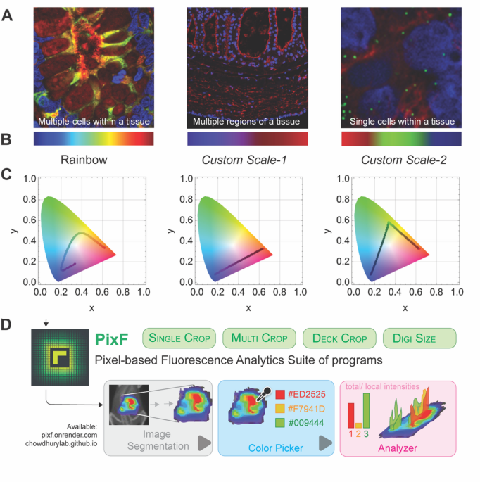
Mapping colorbars to chromaticity and fluorescence imaging bridges raw data with meaningful visualization. Bioimaging supports numerous biological discoveries, yet different techniques utilize distinct wavelength ranges to probe cellular components (Fig. 1A). Accurately visualizing this spectral information is crucial for interpretation. This study investigates the mathematical relationship between colorbars (Fig. 1B), chromaticity plots (Fig. 1C), and fluorescence intensity data mapped onto the RGB color space (Fig. 1D). While PixF was tailored to serve the purpose of this work, its generalizability as a reliable image processing platform when compared to ImageJ (and others) needs comprehensive benchmarking. Benchmarking against legacy tools like ImageJ is a lengthy endeavor. Therefore, preliminary soft benchmarking evidence for PixF was provided in the supplementary data (Figs. S2, S3, and Table S4)29.

PixF workflow—color scheme analysis, chromaticity mapping, and image segmentation modules. (A) PixF has been built to learn multiple color schemes used for different biological imaging experiments spanning scales of life. (B) By reasoning over the data, PixF can identify a color palette (albeit without directionality) where the user should indicate which end of the spectrum is high and which is low. (C) A chromaticity analysis enables projecting the travel of a color palette from a given image on the visible spectrum (convex hull). This is important for calculating the definitions of neighborhoods for a given color in the image. For example, Rainbow and Custom Scales have a larger travel and hence have a larger neighborhood for each color in comparison to FuchsiaTones. This means sensitivity towards variance in pixel-level intensity for FuchsiaTones must be stringent during PixF analysis. (D) Overview of the image segmentation, color picker (without a palette), and analyzer modules in PixF.
Colorbars and chromaticity
Colorbars (e.g., ‘Rainbow’) map numerical data to colours via defined colormaps. Chromaticity diagrams, such as the horseshoe-shaped plot (Fig. 1C), offer a framework for understanding this mapping. These plots represent perceivable colors through hue (color) and saturation (intensity). A colorbar sample points along specific paths in this chromaticity space. For example, the “Rainbow” colormap traverses a curved path encompassing hues from violet to red with increasing saturation towards the center.
Bioimaging and spectral ranges
Bioimaging techniques rely on fluorescence, where molecules emit light upon excitation at specific wavelengths. Different methods target various fluorophores with unique excitation and emission spectra. Confocal microscopy often utilizes 400–700 nm wavelengths, while Raman spectroscopy probes vibrational modes in the near-infrared range (700–1400 nm). Tools like PixF incorporate spectral spans to interpret fluorescent intensity data accurately. For example, applying a “Rainbow” colormap to Raman data may misrepresent information by exceeding the utilized wavelength range.
Mapping fluorescence to RGB
Fluorescence intensity data, measured in arbitrary units, requires conversion into RGB values for visualization. This mapping may use linear or non-linear functions to enhance contrast or emphasize features. Selecting an appropriate colormap significantly affects how fluorescence intensity variations translate into visual representations. While intuitive colormaps like “Rainbow” may lack precision, scientifically optimized colormaps such as “Viridis,” “Inferno,” “Plasma,” and “Magma” (Matplotlib, v3.9.2)30 provide perceptually accurate data visualization. Custom colormaps tailored to specific bioimaging applications further enhance interpretability.
3D bar plots for spatial molecular expression
The Python-based parsing module within PixF analyzes fluorescent images to quantify and visualize molecular expression across tissues. Images comprise red, green, and yellow channels, where yellow denotes overlapping red and green fluorescence regions. PixF splits images into individual channels, maps each pixel’s location to the tissue region, and generates 3D bar plots. These plots map intensity values onto a normalized RGB scale, visually representing the spatial intensity of molecular expression in three dimensions.
3D bar plots facilitate the identification of differential molecular expression, highlighting tissue regions where one marker dominates at a pixel level. This capability uncovers spatial patterns of molecular activity, offering insights into viral infection mechanisms and tissue-specific entry points. Such quantifiable biological insights are critical for understanding how viruses affect host organs and tissues differently.
Availability of PixF through a web-based platform
PixF is a freely accessible web-based tool featuring an intuitive graphical user interface (GUI) that enables users to upload fluorescence data (red, green, and blue channel values) alongside acquisition details, such as excitation and emission wavelengths. The platform applies mathematical transformations to map data into a relevant chromaticity space based on excitation/emission information, supports user-defined adjustments like mapping function fine-tuning and colormap selection optimized for specific applications, and generates high-resolution, publication-quality visualizations. By bridging raw fluorescence data with interpretable visual outputs, PixF democratizes access to advanced bioimage analysis tools, fostering deeper insights into bioimaging experiments. The tool is available at https://pixf.onrender.com/.
Statistical analysis
Respiratory and intestinal tissues from three animals and representative images were chosen and analyzed based on consistent staining intensity and structural integrity across replicates, as recommended31,32. Statistical analyses and plots were performed using GraphPad Prism® 10.6.0 (GraphPad Software Inc.). Total lectin staining intensity values were log10-transformed prior to analysis. A two-way ANOVA followed by Tukey’s post hoc multiple comparisons test was used to evaluate differences in the labeling levels of three sialic acid (SA) types within the same tissue, as well as the labeling of a single SA across different tissues. For the individual immunofluorescence assays, log10-transformed total intensity values were analyzed using one-way ANOVA (within each receptor type), followed by Tukey’s post hoc test to compare labeling levels across different tissues. For all analyses, a p-value < 0.05 was considered statistically significant.